Is the shape below rotated to the right or the left?

How about this one?

The process by which our nervous system converts physical stimuli to neural activity is referred to as sensation, but making sense of that information is referred to as perception. The field of studying how physical differences in stimuli affect perception is called psychophysics, and one of the research techniques for studying this is signal detection theory. The ideas behind signal detection theory occur frequently in user research, so they’re worth reviewing here. Whether we’re trying to detect whether a product change influences user satisfaction, or trying to measure preference for a product design, having a good understanding of signal detection theory serves as a foundation for future research method discussions. Most importantly, the same scientific rigors used to measure perceptions can be used to measure preferences. After all, isn’t preference just a type of perception, as in, perceived benefit, or perceived value?

The first core concept in signal detection theory is the idea of a decision variable. The premise here is that as certain features of the physical stimulus change, there is a corresponding change in the neural representation of that stimulus. Simply put, when stimuli change, our brains process the stimuli differently. When we make judgments about physical stimuli, we’re actually making judgments about the neural activity associated with those stimuli. There’s been a great deal of research studying what the “neural correlates of a decision variable” are for different types of decisions. Regardless of what brain activity might correspond to a decision variable, it’s assumed that given the exact same stimulus, there’s going to be some variation in the corresponding decision variable. Further, it’s assumed that the variance in decision variables from one presentation of the stimulus to the next will be normally distributed (i.e. bell curve, or Gaussian distribution).

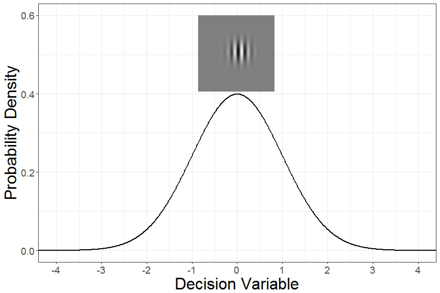
The shapes shown above are called Gabor patches, and they’re often used in studies of visual perception because they’re precisely defined, and different aspects of the shape can be changed independently (e.g. frequency, angle, contrast, size). The decision variable distribution when a vertical Gabor patch is shown should look something like this:

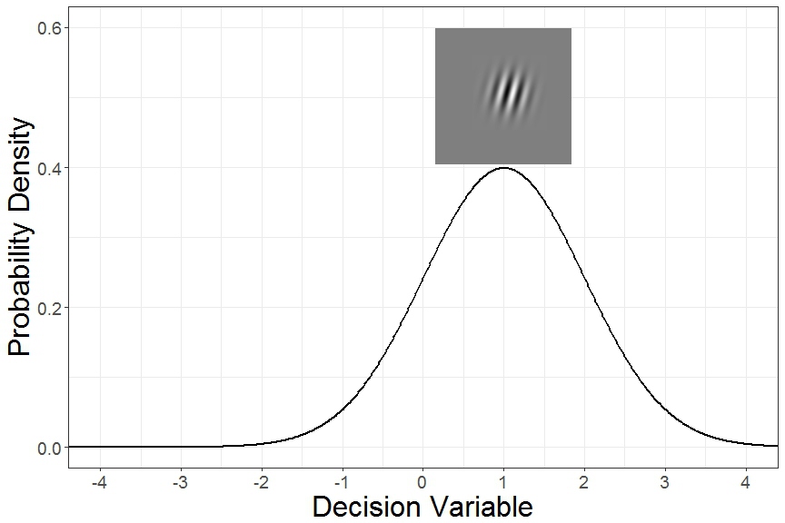
Similarly, if a Gabor patch is rotated slightly to the right, the corresponding decision variable distribution might look something like this:

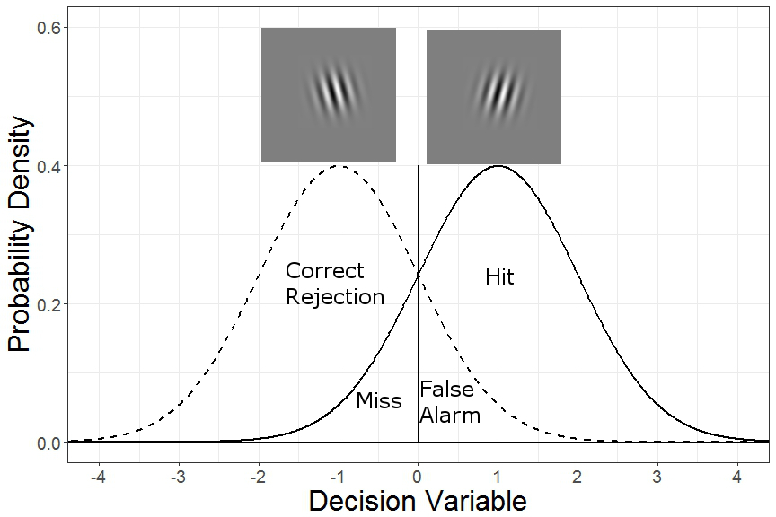
The next core idea of signal detection theory is the criterion. The idea is that when the decision variable is above a certain criterion, we should respond “right”, and if it’s below a certain criterion, we should respond “left”. But some of the time we’d choose the incorrect rotation by chance alone. In classic signal detection theory experiments, scientists were studying the limits of human perception and so were measuring whether people could see a dim flash of light, or hear a faint tone. When a person correctly detects a signal (flash of light or dim tone), this is called a “Hit”. Similarly, when they correctly say that no signal was present, this is called a “Correct Rejection”. Incorrect guesses that a signal is present when it really isn’t are called “False Alarms”, and guessing a signal was absent when it really wasn’t are called “Misses”. If we arbitrarily define rightward angled patches as our “signal” distribution, the different types of responses can be seen below.

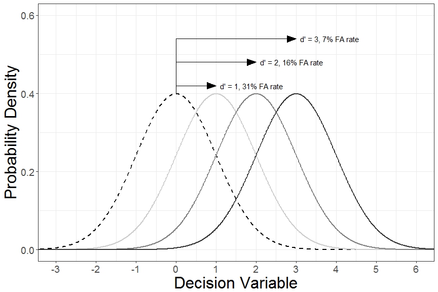
Now, here’s the cool thing. Because we’re assuming that underlying decision variable distributions are normally distributed, we can make inferences about how far apart the different distributions are by looking at the patterns of Hits and False Alarms. Given enough trials, we know how far the “Right” decision variable distribution is shifted upward or rightward relative to the criterion by the percent of Hits. Similarly, we know how far the “Left” decision variable distribution is shifted downward or leftward relative to the criterion by the percent of False Alarms*. For example, a hit rate of 84% means that 84% of the “Right” decision variable distribution must be above the criterion, or in other words, the criterion is located 1 standard deviation below the mean of the “Right” decision variable distribution. Similarly, a False Alarm rate of 16% means that 16% of the “Left” decision variable distribution must be above the criterion, or 1 standard deviation above the mean of the “Left” decision variable distribution. By definition, detectability (and disriminability) is defined by how many standard deviations the underlying decision variable distributions are from each other. This metric is called d-prime (or d’). This value is relatively straightforward to calculate. In Excel, use d’ = normsinv(hit rate) – normsinv(false alarm rate). In R, d’ = qnorm(hit rate) – qnorm(false alarm rate).

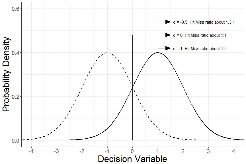
So far, we’ve only considered cases where we’re unbiased in our guesses whether the Gabor patch is rotated left or right. Calculating where in the decision variable distribution the criterion is located is found in Excel by c = 1/2(normsinv(hit rate) + normsinv(false alarm rate)) and in R by c = 1/2(qnorm(hit rate) + qnorm(false alarm rate)). Notice that when we’re unbiased in our responses, this value equals zero. If we’re more likely to favor responses of “Right”, False Alarms happen more frequently than Misses, and c becomes negative. Similarly, if we’re more likely to favor “Left” responses, Misses occur more frequently than False Alarms, and c becomes positive.

But, what if leftward rotated patches are shown 3 times more often than rightward patches? Or suppose that we’re given $1 for each correct “Left” response (Correct Rejection) but are given $2 for each correct “Right” response (Hit). In these cases, in order to maximize the amount we earn or the adjust our guess because of a different base rate of leftward vs. rightward rotated patches, it would make sense to have a different internal criterion. In fact, because we’re assuming that decision variable distributions are normally distributed, if we know the d’ of the stimuli being tested, then the optimal placement of where the criterion should be placed could be calculated. The figure below shows examples of different criteria.

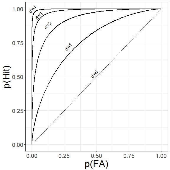
Systematically manipulating the response criterion and evaluating the corresponding changes in Hit and False Alarm rates can be used to create a receiver operating characteristic (ROC) curve. It’s worth noting that this also serves as an empirical test that the underlying distributions are normally distributed, as assumed. The figures below show examples of ROC curves for different underlying decision variable distributions.

This article introduced a number of concepts that can become important when doing user research. If two product features are slightly different, how easily can users detect those differences? How much data must we collect for us to be confident that, if there really was a difference, we would have been able to detect it? Moreover, what is the relationship to perceived difference and preference? Did users to your website notice the different shaped “Buy Now” button? Did they notice it and just not care? To what extent do users make perceptual judgments about their own internal states when deciding which product concept they prefer? Much of research comes down to these types of questions and our ability to compare different probability distributions against each other, in conceptually much the same way that signal detection theory does.

*A signal detection purist would point out that in this experiment, both the rightward distribution and the leftward distribution could be modeled as being compared to a third internal “neutral” or vertical distribution on each individual trial. As a primer to signal detection theory, we arbitrarily define the “left” distribution as the “noise” distribution for simplicity.